As machine learning continues to evolve, transforming the various industries it touches, it has only begun to inform the world of audit. As a data scientist and former CPA Auditor, I can understand why this is the case. By nature, auditing is a field that focuses on the fine details and investigates any exceptions, while machine learning typically seeks to extrapolate broad patterns. Where auditing focuses on analyzing historical events, machine learning solutions tend to predict future events. Lastly, most auditors lack the necessary education or coding skill set to proficiently experiment with machine learning in their work. Below I will demonstrate how we used machine learning to solve one particular auditing problem at Uber, and by extension how our methodology and architecture can be leveraged to address other data problems in the greater audit industry.

“Hey Internal Audit, tell me something that I do not know?…”

Cash intermediaries (also “Agents”) are established, third-party vendors, which the Company asks to act as an agent between the Company and other vendors. Why would a company need such intermediaries? Your business may operate in certain countries where some of the local vendors from whom you need products and services are not able to operate through your P2P processes and systems. For example, suppose you want to buy a batch of flowers, but the florist cannot go through the company’s Accounts Payable system. An established Agent (actually on-boarded on the Company’s P2P) would buy that batch of flowers for you from the florist with cash. Then, the Agent would add that expense item to its next bill (for its own services) and the Company would reimburse that Agent.

This is just a simple and benign example. Though the use of these Agents is not illegal per se, the uncontrolled proliferation of such transactions is prone to several risks. For example, how do you know that the florist is selling legally? How do you know the actual price of the flowers? Is the Agent charging the Company back correctly? Do the florist and the Agent have a conflict of interest? Are you using the Agent to bypass your own conflict of interest with the florist or to mask kickbacks, bribery, or the fact that this type of expense is simply not permitted?

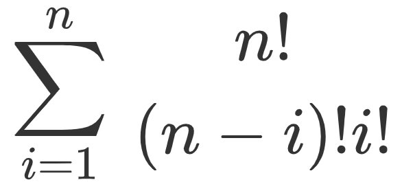
In the case of Uber, historically, these Agents were manually engaged by local teams worldwide, and there was no visibility into what was happening. We knew such Agents existed because we had completed a couple of fraud investigations revolving around such cases. However, a number of questions remain: how many vendors are we actually using as Agents? In what types of cases are those Agents used? And geographically, where are these Agents used and how much are being processed? Because there were no systemic precedents for identifying these Agents, our preliminary approach to finding them was to inquire with local teams and build a heuristic approach. Then, we translated our understanding into SQL. However, this approach proved to be highly limited. We believe that there are much more complex relationships between Agents and non-Agents, particularly regarding the potential number of features involved. It is not feasible to build a number of logic gates in SQL equal to the number of unique combinations of each feature, or mathematically, (where n is the number of features available in our Spend Management platform), so we hypothesized that using machine learning could help remedy the problem.

To reiterate, we had just a small sample of labeled data (confirmed Agents from local teams). As for the data source, we used tables that ingested the data in our Spend Management platform to obtain the data and features, such as transaction type, description, amount, currency, etc.

Challenge Accepted

Data Availability:

One of the biggest roadblocks was that we did not have a lot of labeled or available data. From our initial inquiry with local teams, we had labeled 47 out of 477 vendors as Agents. As data scientists, we know that these samples are not sufficient to train any model. To increase the number of records in the population, we expanded our data set from vendors to purchase orders (POs). See the Model Design section for details about how this was done.

Data Labeling:

Labeling focused primarily on vendors that were, in fact, Agents. On the flip side, we could not confirm the accuracy of negative labels. Auditors know that positive-confirmations (when someone explicitly tells you whether or not something is correct) are superior to negative-confirmations (when someone is asked to reply only if something doesn’t look right), aside from the added work for the confirmations. To tackle this problem, we should use a recall score as a metric in every evaluation. Depending on the business problems you face, you may want to prioritize other metrics.

The Research Journey

Dimensionality Reduction

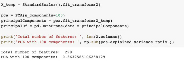
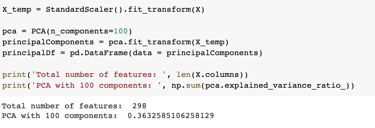
Once we dummy encoded (or one-hot encoded) our categorical features, such as currency and department, we ended up with almost 300 features. This is where we considered dimensionality reduction, which typically yields faster training times, better model performance, or both.

We used Principal Component Analysis (PCA) with 100 components, resulting in only 36% of the variances being explained. Because a third of the data gave us just slightly over a third of the explained variance, it appears that we would need to use all the features in order to capture a complete picture, and so we pushed all available features through our models.

Experimentation

Model v1 Design and Results

In our first iteration, we used K-nearest neighbors (KNN). The features included the USD amount and the presence of four high-risk transaction types. In the PO-level predictions, the accuracy was around 92% for K∈{1, 3, 5, 7, 9}. In the vendor-level predictions, the maximum accuracy achieved was 88%. For a simplistic model with minimal features, it seemingly performed well. However, keep in mind that the data is heavily imbalanced in the ratio of approximately 1:10; therefore, accounting for the baseline null-accuracy of 91%, we cannot say that this model did much of anything. Null accuracy is if the model simply predicts the majority class every time. Therefore in our 1:10 imbalanced dataset, the model would predict accuratelytimes, or 91%, if it only predicted 0’s.

Lesson Learned: When evaluating the model performance, make sure to evaluate the model against a baseline. In our case, we used the null accuracy.

Model v2 Design and Results

In our second iteration, we used Random Forest Classifier on only PO-level data. The purpose of this was primarily to train a fast model that would provide us with information about feature importance and whether it made sense to classify these features as such.
We also observed a 95.9% average accuracy score through a 4-fold cross validation. Breaking that down, we ended up with 95.8% precision and 97.5% recall. While the results looked promising, we had to be cautious about our evaluation. To start, we assumed positive labels for all transactions transacted by a labeled vendor. Somehow, we had to dampen this factor. Furthermore, we needed predictions on vendors, not predictions on transactions. We also had to infuse vendor-level features into our model.
Upon a deeper dive into the predictions, the preliminary results from this Random Forest model appeared questionable. When we looked at all transactions for a predicted vendor, for example, we couldn’t logically say that the prediction had attributes similar to an Agent.

Lesson Learned: Although the predictions may well be above the baseline, it’s also important to look back at the data from which the model generated those predictions. Also, keeping our objective in mind, we wanted to predict individual vendors, not transactions.

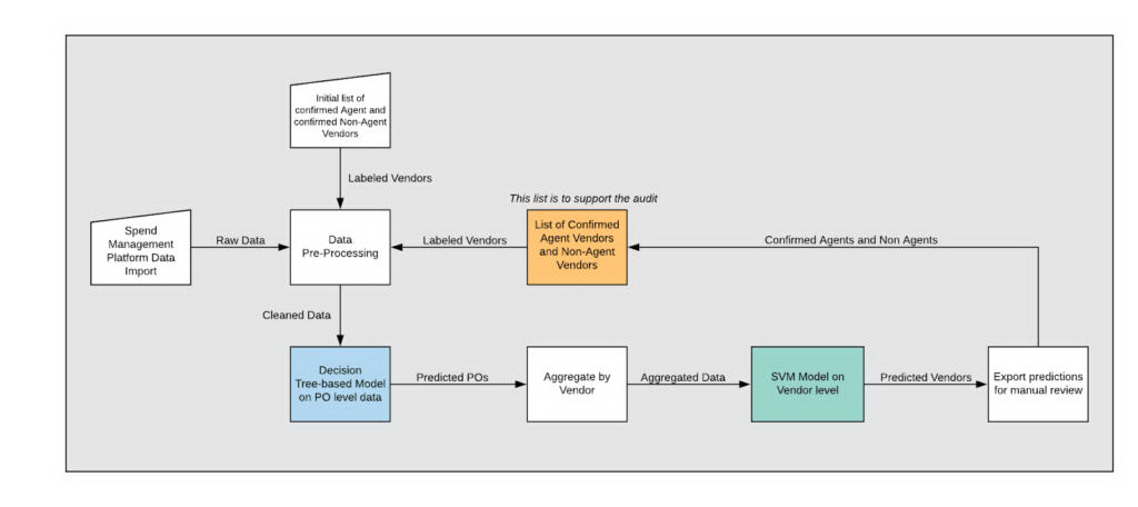
The Final Architecture Design

To accommodate the paucity of both labeled and available data, we designed a dual-model architecture.

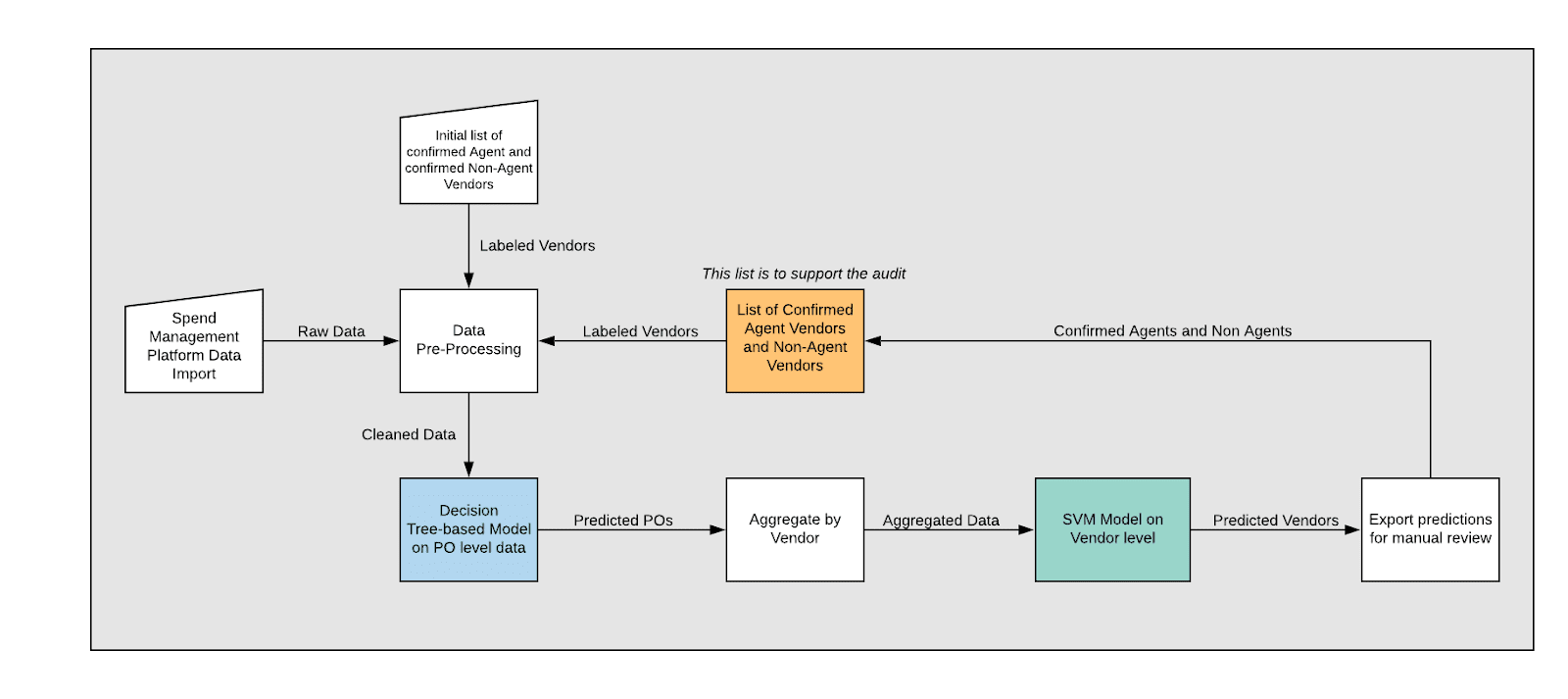
Our final architecture is built to use features in both transaction-level data and vendor-level data. This could be achieved only by using a dual-model architecture, in which one model depends on the predictions of the previous model.
First, we built a tree-based model, whether Random Forest or Gradient Boosted Decision Tree. Both GBDT and Random Forest models are tuned prior to deployment. This is the first model; it will attempt to make predictions based on transaction-level data, such as currencies, departments, amounts, and descriptions. We will refer to this prediction as the first-level guess on which transactions appear suspicious. In tuning the first models, we optimized for the recall score, as we wanted to minimize false negatives.

Using only a single-model architecture has logical and technical drawbacks. First, our objective is to predict Agents, not transactions. The single model would attempt to predict transactions, not Agents. In addition, there are features that cannot be encoded in the transaction-level data, such as the number of distinct commodity types per vendor. Therefore, after this first-level prediction, the next step was to aggregate the results by vendor. We chose to count the number of unique entities with which the vendor engaged in transactions (for example, Uber and Uber BV are different entities), count the number of unique transaction types for each vendor, and take the average of predicted transactions per vendor. For example, if a vendor had 10 transactions and 8 of them were predicted (not labeled) by the first model, this vendor would receive a 0.80 in the aggregation.

Finally, the Support Vector Machine (SVM) model would use all the features to make a final prediction. In tuning the SVM models, we optimized for the balanced-accuracy score, to account for the imbalanced data.

Why didn’t we use Naive Bayes? This is because we have no idea what the prior probabilities are. Remember, our labeled data is simply a batch of hand-selected vendors. We don’t know if they constitute 5%, 10%, or 50% of all vendors or transactions. Therefore, we don’t have any grounds to use Naive Bayes.

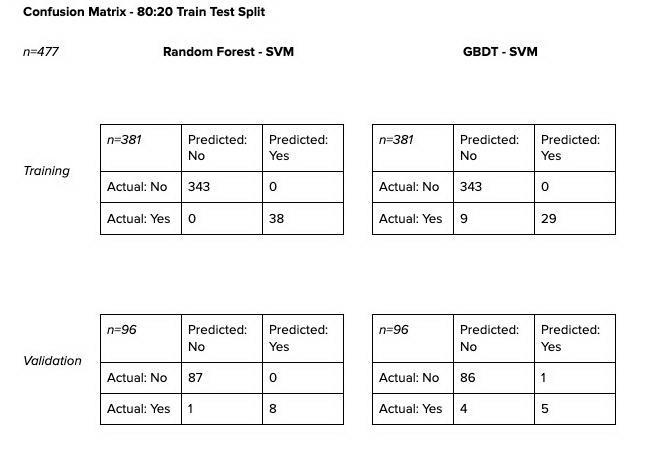
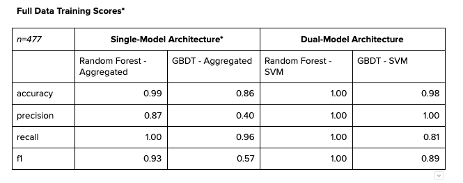
Model Performance

The tables above are the training and validation scores of vendor data in an 80–20 split. Because the number of positive labels were very small, the data was stratified when split.

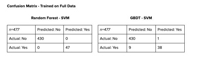
For reference, below is the confusion matrix for after the model is fitted to the entire dataset.

The confusion matrices show promising results. With such small samples, however, we must be very careful about how we evaluate those results. While Random Forest-SVM might seem to have outperformed its GBDT-SVM counterpart, we cannot be quick to dismiss GBDT-SVM altogether.

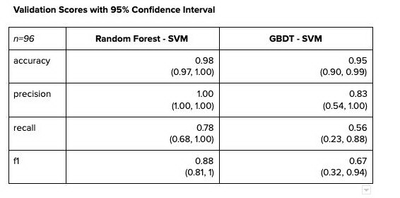
Following are the validation scores with their 95% confidence intervals. Despite the significant differences between point estimates for each statistic, the confidence intervals between the two models actually overlap quite a bit. As we deploy the model into live production and receive more inputs to train, the confidence intervals will become narrower and the point estimates will become more accurate.

If we must evaluate the results of single-model architecture against dual-model architecture, it would be sensible to take the results of the transaction-level predictions and aggregate them by vendors. For benchmarking, if any of the vendors ever had a positive prediction, we would assume that the vendor was a predicted Agent. This method might seem extreme, but realistically, it’s how we would use the predicted results to investigate suspected vendors if we were to only predict on transactions.

Conclusion

In evaluating which model is best, we used the validation scores in Table 3 above as the benchmark by which to make a determination. Given these results, we deployed Random Forest-SVM architecture as the final architecture, not only for its performance, but also for the exponentially faster training and hyperparameter tuning speeds. A Random Forest algorithm can perform a RandomSearchCV in a matter of minutes, whereas GBDT takes over 6 hours to tune. Granted, the Random Forest may have overfitted, but it’s difficult to assess given the current data size. However, as new data comes in, we will need to retain and retune the model, and re-evaluate accordingly. In the meantime, we extracted a handful of vendors based on the model’s prediction and supported the audit with more robust evidence to quantify the problem at hand.

With the help of this project, we were able to more confidently present a full lay of the land to management, answering questions such as how many Agents per country, number of transactions, total cash paid, evolution over the past three years, and use cases. This allowed us to shed light on an issue of which management was not previously aware, as well as providing us with great insights as to how we could engage the right leaders to resolve a business risk. The methodology developed here can be leveraged for other audits as well, and merits further research.